Custom PyMC Models in CausalPy#
CausalPy provides a flexible modelling layer that can be customized at two levels, depending on what you need to change.
Most customization can be achieved without writing a new model class. The Prior system lets you change both parameter priors and the likelihood distribution on any built-in model. When you need to change the model’s structure — how the mean function is computed, adding latent variables, or using non-standard parameterizations — you can subclass PyMCModel and implement a single build_model() method. Your custom model then works with all of CausalPy’s experiment classes, plots, and effect summaries out of the box.
import numpy as np
import pandas as pd
import pymc as pm
import pytensor.tensor as pt
from pymc_extras.prior import Prior

import causalpy as cp
from causalpy.pymc_models import PyMCModel
%load_ext autoreload
%autoreload 2
%config InlineBackend.figure_format = 'retina'
seed = 42
Level 1: Customization via the Prior system#
The built-in models (such as LinearRegression) delegate both their parameter priors and their likelihood to the Prior class from pymc_extras. This means you can change not just the priors on coefficients, but the entire likelihood distribution — all without subclassing.
Changing parameter priors#
Pass a priors dictionary when constructing the model to override defaults:
model = cp.pymc_models.LinearRegression(
    priors={
        "beta": Prior("Normal", mu=0, sigma=10, dims=["treated_units", "coeffs"]),
    }
)
Changing the likelihood distribution#
The likelihood is controlled by the "y_hat" prior. For example, to use a Student-t likelihood for robustness to outliers:
model = cp.pymc_models.LinearRegression(
    priors={
        "y_hat": Prior(
            "StudentT",
            nu=4,
            sigma=Prior("HalfNormal", sigma=1, dims=["treated_units"]),
            dims=["obs_ind", "treated_units"],
        ),
    }
)
This works because LinearRegression.build_model() calls self.priors["y_hat"].create_likelihood_variable(...), which creates whatever distribution you specify. See the Comparative Interrupted Time Series: a geo-experimentation example notebook for a complete worked example using a Student-t likelihood.
Tip
Before writing a custom model class, check whether the Prior system can already do what you need. Changing priors and likelihoods covers many common use cases.
Level 2: Subclassing PyMCModel#
When the Prior system is not enough, you can subclass PyMCModel. This is required when you want to change:
The mean function: How
muis computed from predictors and parameters (e.g.,mu = exp(X @ beta)instead ofmu = X @ beta)Latent variables: Adding hidden variables not in the standard beta/sigma parameterization
Custom error structure: Correlated residuals, heteroscedasticity where sigma depends on covariates
Non-standard parameterizations: Anything beyond what patsy formulas and the Prior system can express
Your custom class needs to implement one method — build_model(self, X, y, coords) — and follow the naming conventions described below. Once you do, all CausalPy experiment classes (InterruptedTimeSeries, DifferenceInDifferences, SyntheticControl, etc.) will work with your model, including their plots, effect summaries, and diagnostics.
The PyMCModel contract#
CausalPy’s machinery (predict, score, calculate_impact, print_coefficients) relies on specific variable and dimension names inside your model. If you use different names, you will get KeyErrors at runtime.
Required variable names:
Component |
Required name |
Used by |
|---|---|---|
Feature data |
|
|
Outcome data |
|
|
Expected value |
|
|
Likelihood |
|
|
Coefficients |
|
|
Noise scale |
|
|
Required dimension names:
Dimension |
Description |
|---|---|
|
Observation index (rows of X and y) |
|
Predictor names (columns of X) |
|
Unit names (columns of y) |
Important
All model code must be wrapped in with self: so that PyMC registers the variables on the correct model instance.
Tip
You can use self.priors["..."].create_variable("...") and self.priors["..."].create_likelihood_variable("...") inside your custom model to get the same prior-override capability that the built-in models have. See the example below.
Example: Log-link regression for positive outcomes#
The built-in LinearRegression uses an identity link: \(\mu = X \beta\). This works well for outcomes that can take any real value, but for inherently positive quantities like revenue or order counts, the counterfactual predictions can become negative — especially during extrapolation.
A log-link model uses \(\mu = \exp(X \beta)\), which guarantees positive predictions and gives coefficients a multiplicative interpretation: a unit change in a predictor scales the outcome by \(\exp(\beta)\).
The implementation below differs from LinearRegression in two ways:
The mean function wraps the linear predictor in
pt.exp()The default prior on
betausessigma=2instead ofsigma=50, since coefficients operate on the log scale where values are typically much smaller
class LogLinearRegression(PyMCModel):
    """Linear regression with a log link function.

    Predictions are constrained to be positive: mu = exp(X @ beta).
    Suitable for positive-valued outcomes such as revenue or order counts.
    """

    default_priors = {
        "beta": Prior("Normal", mu=0, sigma=2, dims=["treated_units", "coeffs"]),
        "y_hat": Prior(
            "Normal",
            sigma=Prior("HalfNormal", sigma=1, dims=["treated_units"]),
            dims=["obs_ind", "treated_units"],
        ),
    }

    def build_model(self, X, y, coords):
        with self:
            if coords is not None and "treated_units" not in coords:
                coords = coords.copy()
                coords["treated_units"] = ["unit_0"]

            self.add_coords(coords)
            X = pm.Data("X", X, dims=["obs_ind", "coeffs"])
            y = pm.Data("y", y, dims=["obs_ind", "treated_units"])
            beta = self.priors["beta"].create_variable("beta")
            mu = pm.Deterministic(
                "mu",
                pt.exp(pt.dot(X, beta.T)),
                dims=["obs_ind", "treated_units"],
            )
            self.priors["y_hat"].create_likelihood_variable("y_hat", mu=mu, observed=y)
Demonstration: ITS with positive-valued outcomes#
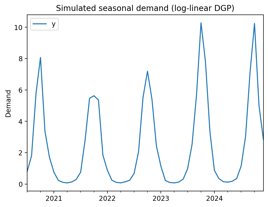
We simulate monthly demand data with strong seasonality. The data-generating process is multiplicative (log-linear), so values are always positive but dip close to zero at seasonal troughs. This is where the log-link model shines — a standard linear model’s credible intervals will extend into negative territory at the troughs, while the log-link model respects the positivity constraint by construction.
rng = np.random.default_rng(seed)
n_pre, n_post = 36, 18
n = n_pre + n_post

dates = pd.date_range("2020-07-01", periods=n, freq="MS")
t = np.arange(n, dtype=float)

# Log-linear DGP: seasonal oscillation that dips very close to zero at troughs
log_y = -0.3 + 2.2 * np.sin(2 * np.pi * t / 12) + rng.normal(0, 0.2, n)
log_y[n_pre:] += 0.3  # ~35% multiplicative lift from treatment

df = pd.DataFrame(
    {
        "y": np.exp(log_y),
        "sin_annual": np.sin(2 * np.pi * t / 12),
        "cos_annual": np.cos(2 * np.pi * t / 12),
    },
    index=dates,
)
treatment_time = dates[n_pre]

df.plot(y="y", ylabel="Demand", title="Simulated seasonal demand (log-linear DGP)");
We use sine and cosine features to capture the annual seasonality. On the log scale, these become multiplicative seasonal effects — exactly matching the data-generating process.
Log-link model#
formula = "y ~ 1 + sin_annual + cos_annual"
result_loglink = cp.InterruptedTimeSeries(
    df,
    treatment_time,
    formula=formula,
    model=LogLinearRegression(
        sample_kwargs={"random_seed": seed, "progressbar": False},
    ),
)
Initializing NUTS using jitter+adapt_diag...
Multiprocess sampling (4 chains in 4 jobs)
NUTS: [beta, y_hat_sigma]
Sampling 4 chains for 1_000 tune and 1_000 draw iterations (4_000 + 4_000 draws total) took 1 seconds.
Sampling: [beta, y_hat, y_hat_sigma]
Sampling: [y_hat]
Sampling: [y_hat]
Sampling: [y_hat]
Sampling: [y_hat]
result_loglink.summary()
==================================Pre-Post Fit==================================
Formula: y ~ 1 + sin_annual + cos_annual
Model coefficients:
    Intercept    -0.38, 94% HDI [-0.67, -0.11]
    sin_annual   2.3, 94% HDI [2, 2.6]
    cos_annual   0.12, 94% HDI [0.0068, 0.24]
    y_hat_sigma  0.49, 94% HDI [0.39, 0.61]
fig, axes = result_loglink.plot()
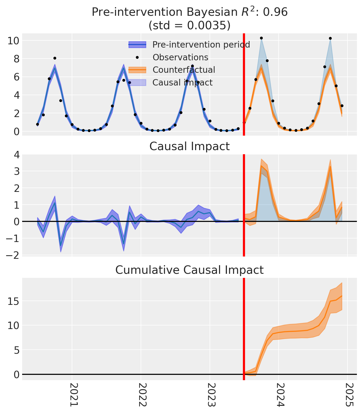
The counterfactual predictions (orange band) stay positive even at the seasonal troughs — the log-link model cannot predict negative demand by construction. The custom model integrates seamlessly with CausalPy’s experiment infrastructure: we get the same summary tables, causal impact plots, and cumulative effect estimates as with any built-in model.
Comparison: default LinearRegression on the same data#
For contrast, let’s run the same analysis with the default LinearRegression (identity link). Notice how the credible intervals extend below zero at the troughs — a prediction that is impossible for inherently positive quantities like demand.
result_linear = cp.InterruptedTimeSeries(
    df,
    treatment_time,
    formula=formula,
    model=cp.pymc_models.LinearRegression(
        sample_kwargs={"random_seed": seed, "progressbar": False},
    ),
)
Initializing NUTS using jitter+adapt_diag...
Multiprocess sampling (4 chains in 4 jobs)
NUTS: [beta, y_hat_sigma]
Sampling 4 chains for 1_000 tune and 1_000 draw iterations (4_000 + 4_000 draws total) took 1 seconds.
Sampling: [beta, y_hat, y_hat_sigma]
Sampling: [y_hat]
Sampling: [y_hat]
Sampling: [y_hat]
Sampling: [y_hat]
fig, axes = result_linear.plot()
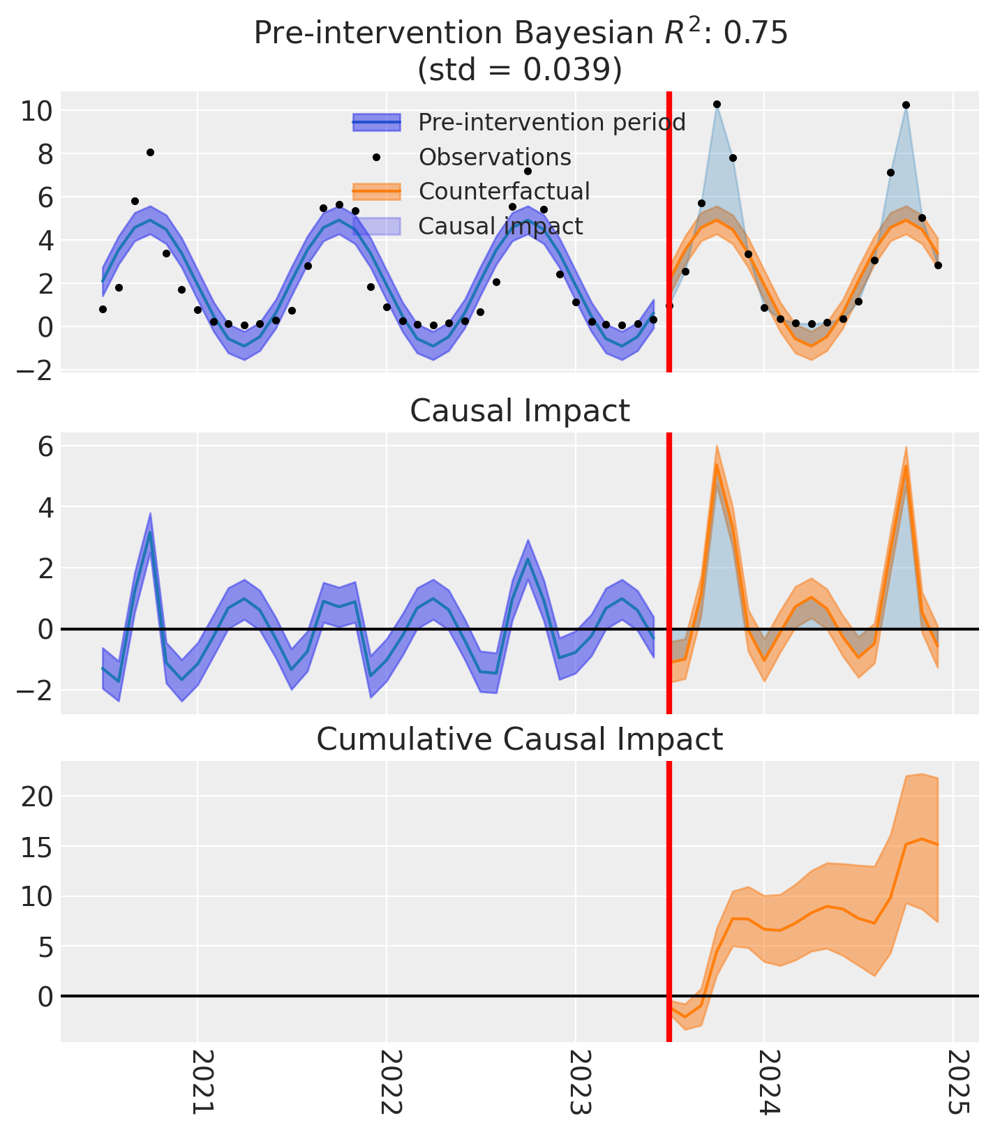
The linear model’s credible intervals dip below zero at the seasonal troughs — physically impossible for demand data. This is the core motivation for the log-link model: when your outcome is inherently positive, the model’s predictions should be too.
Common pitfalls#
Wrong variable names. If you name your deterministic "mean" instead of "mu", or your likelihood "obs" instead of "y_hat", you will get a KeyError from predict() or calculate_impact(). Always use the names from the contract table above.
Missing with self:. Forgetting to wrap your model code in with self: means PyMC creates variables outside the model context. This leads to empty models that silently produce incorrect results during fitting.
Prior scale mismatch. When changing the mean function (e.g., log link), remember that coefficients operate on a different scale. The default LinearRegression priors assume identity-scale coefficients — these will be far too wide for a log-link model where coefficients represent log-scale changes.
Missing treated_units coordinate. The base class expects a "treated_units" dimension. If your data has a single unit, add a default:
if coords is not None and "treated_units" not in coords:
    coords = coords.copy()
    coords["treated_units"] = ["unit_0"]